Crowd Counting using Deep Learning

Crowd Counting with Deep Learning

Table of Contents

1. Business Problem
2. Introduction of Crowd Counting Problem
3. Deep Learning Formulation of Business Problem
4. Business Objectives and Constraints
5. Dataset Analysis
6. Evaluation of Performance Metrics
7. Exploratory Data Analysis
8. Data Pre-Processing
9. Preparing Data for Modeling
10. Apply Deep Learning Models
11. Conclusion
12. Future Work
13. GitHub Repository
14. References

1. Business Problem

Predict the number of people in the given image.

2. Introduction

Crowd counting problem is to count or estimate the number of people in each image. This will mainly be useful in real-life public monitoring such as Surveillance and traffic control. This will help to prevent calamities stampede could be alleviated, which make great sense for public security. And could be helpful to understand the crowd behavior which could help to improve design of built environment and increase public safety.

Other than public safety measures, Crowd counting problem will also help in commercial business such as malls, stations, bus transportation. This will help to plan and improve the sales businesses day to day basis depends on the number of people visit.

Images will be usually monitored and captured with the help of Close Circuit Television (CCTV).

There are two kind of images which are Sparse Images and Dense Images.

Sparse images refer to a less number of people in a given image. Dense Images refers to huge number of people in each image.

Crowd counting is very difficult mainly in dense images due to following reasons.

1) Irregular distribution of objects

2) Often Clutter

3) Occlusions

4) Overlap

5) Pose Estimation

Since it is very hard to count / monitor the crowd gatherings by the operators continuously, somehow need to automate the process by implementing some techniques to identify the crowd count on each image to minimize the human involvement and plan better to improvise the sales, public safety etc.,

3. Deep Learning Formulation of Business Problem

There are many techniques to estimate the people count in a given image. Some of the techniques are as follows with limitations.

1) Detection Based Approach:

This is the first early technique found mid of 2006 year to estimate the person counts. In object detection-based counting, the object detectors are trained to localize the position of every person in the crowd for counting.

Limitations:

- It is difficult to count the exact number of people if the input is dense image due to most of the target objects are seriously obscured in highly congested scenes.

2) Regression Based Approach:

This technique found in the mid of 2008 year. This will estimate the crowd count by carrying out regression between image features and crowd size. This model will work pretty good on high density images. However, it has some limitations on high density.

Limitations:

- Performance degradation on high density images

- Well work for only for low density images where all the people parts are visible clearly.

3) Density Estimated Based Approach:

Earlier approaches don’t consider spatial information. However, Density Estimated approach focuses on density by mapping between local features and object density maps, there by incorporating spatial information in the process. Linear mapping and non-linear mapping will be used to calculate Density calculations.

4) Deep Convolutional Neural Network (CNN):

CNN are advanced technique mainly used for image recognition, image classification, Object detection's, face recognition etc.,

CNN image will take input as image and predict the people count of each image. CNN will be based on estimating the density map over the images.

4. Business Objective and Constraints

• Low Latency requirement
• Errors can be very costly

5. Dataset Analysis

Let’s analyze more on the provided dataset to apply Deep learning techniques.

Please refer below dataset files and columns/features in dataset

1. Images.npy: This file is a NumPy file which contains 2000 different RGB images of 480X640 pixels.
2. Frames Folder: This folder contains 2000 RGB images files with 480X640 pixels.
3. Label.csv: This file contains following columns.

Id: This column contains 2000 rows with id.

Count: This column contains people count per image against each “id” column.

4. Labels.npy: This is a NumPy file which contains the count of every image (rows and index are ordered)

Note: Lets consider “Images.npy” and Label.csv files for this case study.

6. Evaluation of Performance Metrics

We will consider people counting task as a regression problem whose input is a RGB images and output is a real value. Hence considering below performance metrics to evaluate the regression model.

1) Mean Absolute Error (MAE): MAE measures the average magnitude of the errors in a set of predictions, without considering their direction. It’s the average over the test sample of the absolute differences between prediction and actual observation where all individual differences have equal weight.

Figure 3: MAE Formula

2) Mean Squared Error (MSE): MSE is calculated by taking the average of the square of the difference between the original and predicted values of the data.

Figure 4: MSE Formula

7. Exploratory Data Analysis (EDA)

Lets perform Data Analysis on the dataset to understand the data.

7.1 Reading Data

Here we will load two different files.

File 1: “Images.npy” which contains list of images.

File 2: “Labels.csv” which contains the people count of each image

Note: Indexing for File 1 and File 2 are same. With the help of indexing, we will merge both dataset further

Lets read “Images.npy” file. There are totally 2000 images are loaded from numpy file. Each image pixel size is 480 X 640 with 3 channels (RGB)

Lets read another dataset called “Labels.csv” file

7.2 Plot “Count” Feature Distribution

Below plot results represents a Bell shape (Gaussian) Distribution. Noticed that, out of 2000 images, People Count lies between 37 to 33 has more number of images.

7.3 Display Images

Lets cross check some of the images by plotting it here. This is to check and confirm that the images and dataset are loaded properly with out having any issues.

Images are properly loaded from .npy file and can able to display it as well.

To analyse the images further, lets segregate the images based on following rules and plot the images. This will help to understand how the people inside images are distributed across.

1. Segregate Low People count Images
2. Segregate Medium People count Images
3. Segregate High People count Images

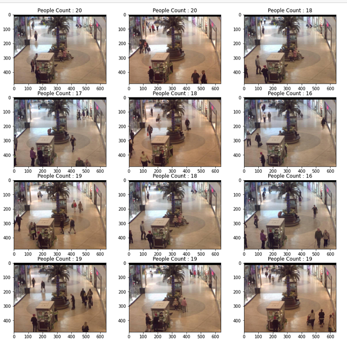
7.3.1 Plot Low People Count Images

Lets consider the images where people count is ≤20 are low people count images.

7.3.2 Plot Medium People Count Images

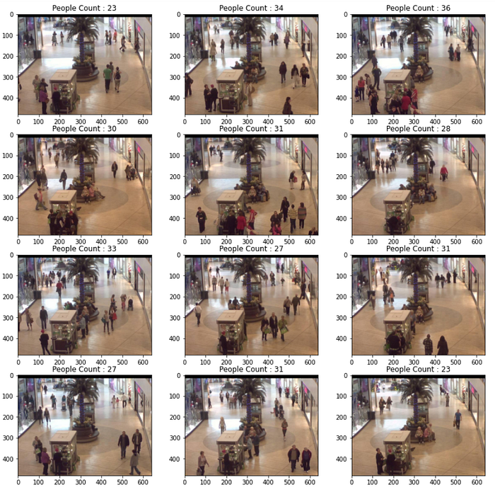
Lets consider the images where people count between 21 and 40 are medium people count images.

7.3.3 Plot High People Count Images

Lets consider the images where people count between 41 and 60 are medium people count images.

8. Data Preprocessing

Lets apply below preprocessing techniques against the images randomly. This will boost Deep Learning models to predict the output precisely.

1. Resize all images to 400X400
2. Apply Flip Left Right on the images randomly
3. Apply Flip Up Down on the images randomly
4. Apply brightness on the images randomly
5. Apply Saturation on the images randomly

seed=(1,2)
def preprocess_image(image,count):
    #image,count = image,count
    image = tf.cast(image, tf.float32)
    image = tf.image.resize(image, [400, 400])  #resizing the image to 400X400 pixels
    image = tf.image.random_flip_left_right(image) #fliping the image left to right
    image = tf.image.stateless_random_flip_up_down(image,seed) #flipping the image upside down
image = tf.image.stateless_random_brightness(image, max_delta=32.0 / 255.0, seed=seed) #Randomly changing the brightness to the images
    image = tf.image.stateless_random_saturation(image, lower=0.5, upper=1.5, seed=seed) #Randomly changing saturation to the images
return image,count

Will apply preprocessing technique on the dataset after splitting the data in to Train and Test.

9. Preparing Data for Modelling

9.1 Prepare Data

Lets build TensorFlow input pipeline using tf.data.

Tf.data: tf.data API enables to build complex input pipelines from simple, reusable pieces. For example, the pipeline for an image model might aggregate data from files in a distributed file system, apply random perturbations to each image, and merge randomly selected images into a batch for training. The tf.data API makes it possible to handle large amounts of data, read from different data formats, and perform complex transformations.

Convert “Crowding_dataset” and “labels_dataset” dataset in to tf.data

9.2 Split Train Dataset

Split the dataset in to train and test with 20 percentage as test data.

val_size = 1600
X_train = final_dataset_tf.take(val_size)
X_test = final_dataset_tf.skip(val_size)

9.3 Preprocessing on Train and Test Dataset

Lets apply preprocessing on Train and Test dataset with the help of map function.

X_train = X_train.map(preprocess_image, num_parallel_calls=AUTOTUNE)
X_test = X_test.map(preprocess_image, num_parallel_calls=AUTOTUNE)

9.4 Configure Dataset Performance

Lets apply following tensorflow parameters for better performance

Cache : It keeps the images in memory after they’re loaded off disk during the first epoch

Shuffle: Shuffle the dataset

Batch: Train the data in batches.

Prefetch: It overlaps data preprocessing and model execution while training

def configure_for_performance(ds):
    ds = ds.cache()
    ds = ds.shuffle(buffer_size=1000)
    ds = ds.batch(batch_size)
    ds = ds.prefetch(buffer_size=AUTOTUNE)
    return ds
X_train = configure_for_performance(X_train)
X_test = configure_for_performance(X_test)

9.5 Display Images After Preprocessing

Lets plot images randomly to crosscheck all the images are preprocessed successfully or not.

We can observe in the following images that, brightness, saturation, flip left right and resizing are applied on the images.

10. Applying Deep Learning Models

Below are the choosen DL Models for the given dataset.

1. According to this research paper, one of the proposed solution would be Compact Convolutional Neural Network. Below are the main objectives of proposed solution.

a. Simple CNN architecture

b. Will contain a smaller number of parameters to improve the performance of a model.

Below is the proposed C-CNN architecture.

Explanation: Input is a image to the CNN following by three parallel Convolution layers with three different sizes of Kernels. All three Kernels will be followed by MaxPooling and convolution layers.

First kernel will be used to pay more attention on large receptive fields. Second kernel will pay attention on dense crowds. Third kernel will pay attention on highly congested crowded scenes. After the extraction process of various receptive fields, the feature maps are merged as feature fusion for follow-up layers to perform down-sampling. We find that using only one layer of convolution is enough to extract different spatial features and could ameliorate the efficiency of feature extraction from multiple branches. This is why the network is faster and accurate.

2. Simple CNN Model which consists of 2 Conv2D layers along with Maxpooling, Batch Normalization and Dropouts.

Lets understand some of the key terms here

Conv2D: Conv2D is a 2D Convolution Layer, this layer creates a convolution kernel that is wind with layers input which helps produce a tensor of outputs

Maxpooling: It helps to down samples the input representation by taking the maximum value over the window defined by pool_size for each dimension along the feature axis

Batch Normalization: Batch normalization applies a transformation that maintains the mean output close to 0 and the output standard deviation close to 1

Dropouts: It’s a regularization technique. It will randomly drop the neurons during training.

10.1 How to apply Deep learning Model

Below is the process to apply Deep Learning models after data is preprocessed and done with train_test split.

1. Initialize Parameters
2. Create a Model (Sequential / Continuous)
3. Define Architecture (layers)
4. Define Optimizer, Metric and Compile Model
5. Train the Model
6. Evaluate the Model

10.2 Model 1: Apply C-CNN Technique

Lets initialize the model and create necessary components based on CNN architecture

from keras import Input, Model, Sequential
#from keras.layers import Conv2D, MaxPooling2D, Concatenate, Activation, Dropout, Flatten, Dense
from tensorflow.keras.layers import Conv2D,Dense,concatenate,Activation,Dropout,Input
# Initialize parameters
input_shape=(400, 400,3)
epochs=50
input_layer = Input(shape=input_shape)
#Define a Model 
#Convolution Parallel layer 1
Conv_Layer_1 = tf.keras.layers.Conv2D(10, kernel_size=(9, 9), padding='same',activation='relu', input_shape=input_shape)(input_layer)
inputlayer_1_pooling = tf.keras.layers.MaxPooling2D(pool_size=(2, 2))(Conv_Layer_1)
inputlayer_1_pooling1= tf.keras.layers.Dropout(0.25)(inputlayer_1_pooling)
#Convolution Parallel layer 2
Conv_Layer_2 = tf.keras.layers.Conv2D(14, kernel_size=(7, 7),padding='same',activation='relu', input_shape=input_shape)(input_layer)
inputlayer_2_pooling = tf.keras.layers.MaxPooling2D(pool_size=(2, 2))(Conv_Layer_2)
inputlayer_2_pooling1= tf.keras.layers.Dropout(0.25)(inputlayer_2_pooling)
#Convolution Parallel layer 3
Conv_Layer_3 = tf.keras.layers.Conv2D(16, kernel_size=(5, 5),padding='same',activation='relu', input_shape=input_shape)(input_layer)
inputlayer_3_pooling = tf.keras.layers.MaxPooling2D(pool_size=(2, 2))(Conv_Layer_3)
inputlayer_3_pooling1= tf.keras.layers.Dropout(0.25)(inputlayer_3_pooling)
#Perform concantenation of all three parallel layers
concatenation_layer = concatenate(inputs=[inputlayer_1_pooling1
                                   ,inputlayer_2_pooling1,inputlayer_3_pooling1
                                  ],name="concat")
#Add 6 convolutional layers as per above architecture
convlayer2 = tf.keras.layers.Conv2D(40, kernel_size=(3,3), padding='same',activation='relu', input_shape=input_shape)(concatenation_layer)
convlayer2_1= tf.keras.layers.BatchNormalization()(convlayer2)
convlayer3 = tf.keras.layers.Conv2D(60, kernel_size=(3,3), padding='same',activation='relu', input_shape=input_shape)(convlayer2_1)
polling_layer3_1= tf.keras.layers.Dropout(0.25)(convlayer3)
convlayer3_1= tf.keras.layers.BatchNormalization()(polling_layer3_1)
polling_layer3 = tf.keras.layers.MaxPooling2D(pool_size=(2, 2))(convlayer3_1)
convlayer4 = tf.keras.layers.Conv2D(40, kernel_size=(3,3), padding='same',activation='relu', input_shape=input_shape)(polling_layer3)
polling_layer4_1= tf.keras.layers.Dropout(0.25)(convlayer4)
convlayer4_1= tf.keras.layers.BatchNormalization()(polling_layer4_1)
polling_layer4 = tf.keras.layers.MaxPooling2D(pool_size=(2, 2))(convlayer4_1)
convlayer5 = tf.keras.layers.Conv2D(20, kernel_size=(3,3), padding='same',activation='relu', input_shape=input_shape)(polling_layer4)
polling_layer5_1= tf.keras.layers.Dropout(0.25)(convlayer5)
convlayer5_1= tf.keras.layers.BatchNormalization()(polling_layer5_1)
convlayer6 = tf.keras.layers.Conv2D(10, kernel_size=(3,3), padding='same',activation='relu', input_shape=input_shape)(convlayer5_1)
polling_layer6_1= tf.keras.layers.Dropout(0.25)(convlayer6)
convlayer6_1= tf.keras.layers.BatchNormalization()(polling_layer6_1)
flatten = tf.keras.layers.Flatten()(convlayer6_1)
#denss1 = tf.keras.layers.Dense(128, activation=tf.keras.activations.relu)(flatten)
output = tf.keras.layers.Dense(1)(flatten)
from tensorflow.keras.models import Model
final_model = Model(inputs=input_layer,outputs=output)
final_model.summary()

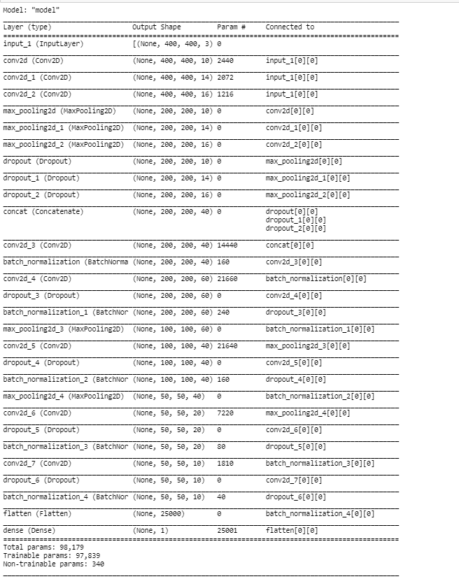
Below is the model summary. This will help to understand the architecture of model in a better way.

Lets Train the model. Have used Callbacks during training the model.

Callbacks: A callback is an object that can perform actions at various stages of training (e.g. at the start or end of an epoch, before or after a single batch, etc). we can use callbacks to :

- Write TensorBoard logs after every batch of training to monitor your metrics

- Periodically save your model to disk

- Do early stopping

- Get a view on internal states and statistics of a model during training etc.,

from tensorflow.keras.callbacks import ModelCheckpoint
from time import time
from tensorflow.python.keras.callbacks import TensorBoard
monitor= tf.keras.callbacks.EarlyStopping(monitor=['mae','mse'],patience=5, verbose=1, mode='auto')
checkpointer = tf.keras.callbacks.ModelCheckpoint(filepath="./Model_1.hdf5",verbose=1,monitor='val_mae',save_best_only=True,save_freq='epoch')
tensorboard=TensorBoard(log_dir="Model1_log1")
Model1 = final_model.fit(X_train,
          epochs=epochs,
          verbose=1,
          validation_data=(X_test),
          callbacks=[tensorboard,checkpointer] 
            )

Predict the output

#Predict the output
y_test_results_model1 = final_model.predict(X_test)
y_train_results_model1 = final_model.predict(X_train)
len(y_train_results_model1)

Plot the Errors

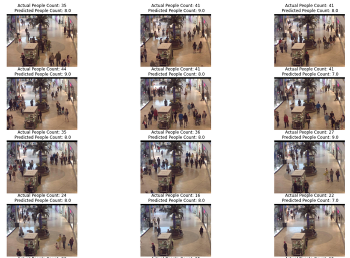
Print images along with predicted output

10.3 Model 2: Simple CNN

Lets initialize the model and create necessary components based on Model 2 architecture

model = tf.keras.Sequential()
model.add(tf.keras.layers.Conv2D(32, kernel_size=(3, 3),
                 activation='relu',
                 input_shape=input_shape))
model.add(tf.keras.layers.Conv2D(64, (3, 3), activation='relu'))
model.add(tf.keras.layers.MaxPooling2D(pool_size=(2, 2)))
model.add(tf.keras.layers.BatchNormalization())
model.add(tf.keras.layers.Dropout(0.25))
model.add(tf.keras.layers.Dense(64, activation='relu'))
model.add(tf.keras.layers.MaxPooling2D(pool_size=(2, 2)))
model.add(tf.keras.layers.BatchNormalization())
model.add(tf.keras.layers.Dropout(0.5))
model.add(tf.keras.layers.Conv2D(128, (3, 3), activation='relu'))
model.add(tf.keras.layers.MaxPooling2D(pool_size=(2, 2)))
model.add(tf.keras.layers.BatchNormalization())
model.add(tf.keras.layers.Dropout(0.25))
model.add(tf.keras.layers.Dense(128, activation='relu'))
model.add(tf.keras.layers.MaxPooling2D(pool_size=(2, 2)))
model.add(tf.keras.layers.BatchNormalization())
model.add(tf.keras.layers.Dropout(0.5))
model.add(tf.keras.layers.Flatten())
model.add(tf.keras.layers.Dense(1))
model.summary()

Below is the model summary

Load the model and predict the output.

Model 2 predictions will be saved in to “y_test_results_model2” variable. We will use the results to perform analysis on image at later stage.

model.load_weights('./Model_2.hdf5')
#Predict the output
y_test_results_model2 = model.predict(X_test)
y_train_results_model2 = model.predict(X_train)

Plot the errors

%matplotlib notebook
import matplotlib.pyplot as plt
import numpy as np
import time
# https://gist.github.com/greydanus/f6eee59eaf1d90fcb3b534a25362cea4
# https://stackoverflow.com/a/14434334
# this function is used to update the plots for each epoch and error
def plt_dynamic(x, vy, ty, ax, colors=['b']):
    ax.plot(x, vy, 'b', label="Validation")
    ax.plot(x, ty, 'r', label="Train")
    plt.legend()
    plt.grid()
    fig.canvas.draw()
fig,ax = plt.subplots(1,1)
ax.set_xlabel('epoch') ; ax.set_ylabel('Mean Squared error/Loss')
# list of epoch numbers
x = list(range(1,epochs+1))
vy = Model_2.history['val_mse']
ty = Model_2.history['mse']
plt_dynamic(x, vy, ty, ax)

Plot some of the images with prediction

Observation:

• Observed that, Loss and mae is reducing for every epoch. But at epoch 50, results are pretty bad.
• Model 2 provided better results when compared with model 1.

Since Model 2 performed well compared with Model 1. Lets consider Model 2 has a final model and perform Post analysis as mentioned below.

• Plot Best and Worst Prediction Images: This will help to identify which images are predicting correctly by our Model.
• Apply Post Quantization: Post-training quantization is a conversion technique that can reduce model size while also improving CPU and hardware accelerator latency, with little degradation in model accuracy. We can quantize an already-trained float TensorFlow model when we can convert it to TensorFlow Lite format using the TensorFlow Lite Converter.

10.3.1 Plot Best and Worst Prediction Images

10.3.1.1 Pick Best Prediction images and populate from model 2

Create a DataFrame with following columns and copy the output from model 2

Test_Actual: Actual People Count of each image

Test_Predicted: Predicted People count from Model 2 of each image

Test_Difference(actual-predicted): Difference of Actual vs predicted of each image

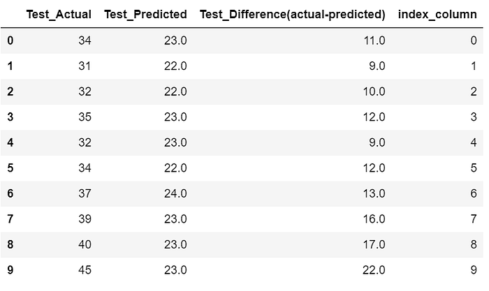
Sort the dataframe ascending order based on “Test_Difference(actual-predicted)” column and store in to another dataframe.

Plot best predicted images

Observation:

Model has predicted correctly (95%) on images which has people count are between 20 and 25

10.3.1.2 Pick Worst Prediction images and populate from model 2

Sort the dataframe in descending order based on “Test_Difference(actual-predicted)” column and store in to another dataframe.

Plot Worst Predicted Images

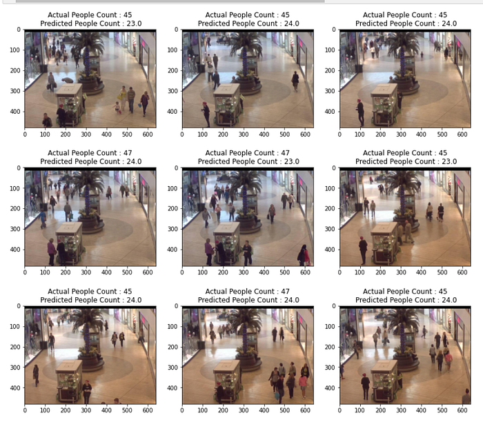
Observation:

Model predicts very badly on the images which has people count >40

10.3.2 Post Quantization (Dynamic range quantization)

Here we will consider Dynamic Range Quantization technique to quantize the weights from floating point to 8 bit precision. This will help 4x reduction in the model size.

Lets apply Post Quantization on Model 2.

Load the saved Model2

Model2_forquantization = tf.keras.models.load_model('Model2.h5')

Convert and save the model to support Quantization

converter = tf.lite.TFLiteConverter.from_keras_model(Model2_forquantization)
converter.optimizations = [tf.lite.Optimize.DEFAULT]
tflite_quant_model = converter.convert()
#saving converted model in "converted_quant_model.tflite" file
open("converted_quant_model.tflite", "wb").write(tflite_quant_model)

Load the converted file

interpreter = tf.lite.Interpreter(model_path="converted_quant_model.tflite")
interpreter.allocate_tensors()

Get input and output tensors details

# Get input and output tensors.
input_details = interpreter.get_input_details()[0]["index"]
output_details = interpreter.get_output_details()[0]["index"]
interpreter.get_input_details()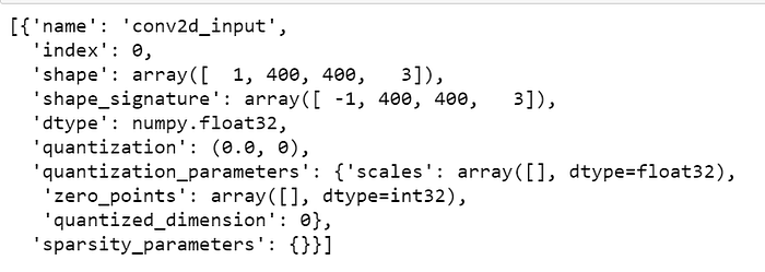

Configure for better performance

X_test_orginal= final_dataset_tf.skip(val_size)
X_test_orginal = X_test_orginal.map(preprocess_image, num_parallel_calls=AUTOTUNE)
batch_size=1
input_shape=(400, 400,3)
X_test_orginal = configure_for_performance(X_test_orginal)
X_test_orginal

Evaluate the Model

y_test_quantization_results_model2=[]
# Run predictions on every image in the "test" dataset.
for img, label in (X_test_orginal.take(50)):
  interpreter.set_tensor(input_details, img)
  # Run inference.
  interpreter.invoke()
  # Post-processing
  predictions  = interpreter.get_tensor(output_details)
  y_test_quantization_results_model2.append(predictions)

Store the results in to dataframe

Model2_Test_results_withQ = pd.DataFrame()
Model2_Test_results_withQ.index +=1601
Model2_Test_results_withQ['Test_Actual']= y_test_count_actual[0:50]
Model2_Test_results_withQ['Test_Predicted_WithOutQuantization']= np.round(y_test_results_model2[0:50])
Model2_Test_results_withQ['Test_Predicted_PostQuantization']= np.round(y_test_quantization_results_model2_final)
Model2_Test_results_withQ['index_column'] = Model2_Test_results_withQ.index+1601
Model2_Test_results_withQ.head(5)

Lets compare results between Pre Quantization vs Post Quantization

Observation:

Prediction with Post Quantization provides a same(nearer) score when compared with Pre Quantization. However, as shown in above plot, prediction with post quantization provides average Pre Quantization score.

Lets Plot the images randomly along with Predicted counts

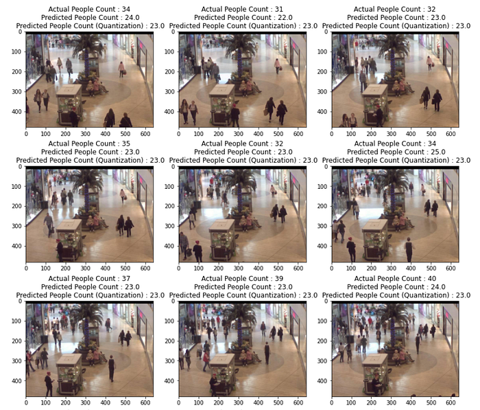
11. Conclusion

• Observed that, Loss and Mae is reducing for every epoch. But at epoch 50, results are pretty bad.
• Model 2 provided better results when compared with model 1.

12. Future Work

1. Sampling the images (which are performed bad) and retrain with CNN model on dataset with sampled images might improve the scores
2. Applying ResNet50, VGG-16 and other models might improve the scores

13. GitHub Repository

Code is available in my GitHub Repository. Kindly have a glance at it.

yavisankar/Crowd-Counting-Problem

14. References

Crowd Monitoring and Localization Using Deep Convolutional Neural Network: A Review

Applied Course

Crowd Counting